I wanted a way to effectively make parallel some of my prebuilt machine learning models. Luckily, the package has this capability inbuilt and it is easy to make massive performance gains in terms of your model runtime. I will show you how in the following article.
Loading imports and finding out my CPU cores
The first step is to load in the required libraries I am going to need:
This loads in the time package, as we are going to create a function to fit the model and time how long it takes to run. I then use sklearn datasets and ensembles to extract the make_classification and RandomForestClassifier – these will make the data described below and fit the Random Forest classifier to the dataset. I will use the os package to get the registered CPUs on my machine, the most important part of this article and then import matplotlib.pyplot for generating some quick plots.
To find out my CPUs I have the following code:
The cpu_count variable stores the number of CPUs your specific machine has, this will vary from machine to machine. This then prints out the number of CPUs. I then create a reserved_cpu variable to hold on to one of the cores for other processing, like graphics. The final_cpu variable just adjusts the CPU count and the following is returned to the console:
Creating a synthetic classification dataset
I am going to create a synthetic classification dataset in scikit learn by using the make_classification function. This is implemented in the code wrapper below:
To explain this:
- n_samples – generates the number of synthetic examples = 10K
- n_features – is the number of columns / features to generate
- n_informative – is used to set how many of the features will be important when we fit the final model
- n_redundant – are those features that will not be used in the data
This is then unpacked to the X and Y variables i.e. the independent variables (X) and the dependent variable (Y).
Create model fit timer function
In the next step we will create the model fit timer function to fit the model and time how long it takes to train:
This run_model function takes in the model you want to fit, the X dependent variables and the Y dependent, or as I call it “the thing you want to predict”. Not sure if this will catch on?
Within this declaration:
- start variable that monitors the current time
- model is the fit function
- end is the end time
- result is the time between when the start and end variables were declared
- A console output is printed to state the time it took to fit the model
- The return statement returns a list ([]) and the fitted model as index 0 and the result of the timer in index 1
Fitting a model on one CPU core
This will use the run_model function we created in the previous step, as well as initialise the model to be fitted:
We initialise the RandomForestClassifier with 500 trees and explicitly declare 1 CPU core to use in the n_jobs parameter. I then store the model in the model_single_list variable, I have named it such, as it returns a list of two indexes – the first is the trained ML model and the second is the run time of the model training. The model trains in:

Fitting a model on all (but one) of my CPU cores
The next model will be initialised in the same way, but this time it will be trained on all (but one) of my CPU cores:
This uses the final_cpu variable we calculated at the head of the script to set the number of parallel jobs to spin up and then the call the run_model function to trigger the model fit timer function. This runs in:

Okay, so we can already see an improvement in the data, it is nearly 5 times faster than the 1 core example.
This is a small dataset, but imagine this performance saving on millions of records and the model having to iterate over this, it soon mounts up. Even more, imagine distributing this over an Azure cloud server and allowing you to distribute over 16 – 32 cores, this would really aid the model training.
Benchmarking by one core increase
The code in the next section trains the model against each of the cores and outputs the results in a list for them to be plotted. I will explain each section of the code in greater depth under this code block:
The variables and components of the model are:
- results_list – this initialises and empty list I am going to use later
- n_cores – this is a list of each core iterated up to 8 cores, as this is the maximum number of cores on my machine
- The for loop uses an iterator variable (model_it) to iterate through the n_cores list
- A model is fitted on each iteration with 500 trees and the n_jobs is set to the current iteration
- the run_model function is ran, which we created earlier, this will fit the model we initialised in the previous step and then store the fitted model as a list, where index 0 is the fitted model and index 1 is the result of the timer function to time how long the model takes to run
- results – stores the timer result
- we then use the append method to append the fit results to the list
- The end return is an appended list of results and run times
I could just print the run times to console, and that is exactly what the function will do, but next, I want to visualise the results of this in matplotlib:
This is a nice little wrapper function that will take the x and y inputs and generate a CPU core benchmark plot. This then produces our benchmark plot:
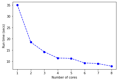
The run time reduces and performance gains start to level out at around 7 cores. We have taken an algorithm that trains in 30+ seconds to one that can be trained in a little over 5 seconds. Such a performance improvement by distributing the load across multiple cores.
What’s next?
The code for this tutorial can be found on GitHub.
In the next article/tutorial I will show you how to optimise sci-kit learn for hyperparameter tuning and cross-validation resampling of the data.
Until then: