
This assumes you know how to programme in Python and know a little about n-dimensional arrays and how to work with them in numpy (don’t worry if you don’t I got you covered).
PyTorch is a pythonic way of building Deep Learning neural networks from scratch. This is something I have been learning over the last 2 years, as historically my go to deep learning framework was Tensorflow.
For beginners to PyTorch it can be daunting to first work with the application as it forces you in the direction of building Python classes, inheritance and tensor and array programming. However, once you start to work with it you start to appreciate the power of PyTorch and how much control it gives you on the creation process of deep neural networks. I have since implemented these frameworks for Natrual Language Processing, Computer Vision, Transformers and audio classification. In this tutorial we will build up a MLP from the ground up and I will teach you what each step of my network is doing.
If you are ready – then let’s dive in! Open your mind and prepare to explore the wonderful and strange world of PyTorch.
The dataset
With this tutorial we will use a dataset from the MLDataR project on classifying whether a person has thyroid disease or not. This uses a number of variables to indicate if thyroid disease is present.
The packages
We are going to need a number of different functions and packages. The first stage is to get all these imported, if they are not installed, then do not concern yourself as I have a requirements.txt file on hand to help you in the supporting GitHub repository:
Here we are using numpy (for array processing), pandas (for working with data frames and series), sklearn for encoding of labels and building up model metrics, torch utilities for working with the input data, torch tensors and other elements of our MLP stack and the time module for timing how long our training loops take.
The data
The data were are going to be using for this PyTorch tutorial has already been preprocessed and consists of all the fields where I have stripped off the row headers.
This is linked to the thyroid data discussed and contains:
- Outcome variable is thyroid_class this is 1=sick and 0=well
- The rest of the outcomes relate to measurements taken associated with thyroid disorders and are explained in the documentation.
The link to the dataset is: https://raw.githubusercontent.com/StatsGary/Data/main/thyroid_raw.csv.
The first stage of the process is to take the data and create a PyTorch readable data object. These are called data loaders and tell PyTorch how to work with the data. This will be defined in the next steps, but to read more about data loaders, see the official tutorial site: https://pytorch.org/tutorials/beginner/basics/data_tutorial.html.
Step one – Building our first PyTorch component – DataLoaders
This is where things get interesting and we will give chunk by chunk into what is happening under the hood.
Creating the data loader to pull in CSV files
Firstly we need to create a dataset class with one input Dataset – this is a specific PyTorch module that works with various types of data. Because we have tabular data, we will need to declare a reader to read in the file from the link above (the raw data stored on GitHub) and then we will do some conversions:
So there are a number of things to explain here:
- We have declared a class which will serve as our blueprint for all other types of data we may want to feed in. You could plug and play this class into your own project and it would work. In this class we pass in an input called Dataset, as I have already explained, this is a special class for dealing with PyTorch objects.
- Next we declare a function using def __init__(). What this means is that when our class is used the first things the class needs are the arguments contained in the function block. Essentially saving, this is what I need when the class is initialised. Within the parentheses we declare two parameters – self and path (the location of the file).
- What is this self parameter? Self represents the instance of the class. By using the “self” we can access the attributes and methods of the class. Essentially, without this you would not be able to access the variables that belong to a class.
- Within the init function we do the following:
- Use pandas to read the csv that is passed to the path
- Set our independent variables to the variable X, but unlike normal functions, you need to make sure you use self.X. This assumed that the data frames values are contained in every column but the last one, this slicing notation says df.values[:, :-1] take all my rows (:) and everything(:) up to the last column (-1).
- The same is done for the outcome variable, bit this time we use the select just the last value [:,-1]
- Next we convert the x value to a floating point value
- We then turn sick and negative our outcome variables into numerical representations using the LabelEncoder() function from sklearn. This just says if it is sick then give it a 1 otherwise 0. This is handy for quickly converting your target variables, as Python would not know what to do with categorical features. Finally, we reshape to make sure it is in the right format for working with an n-dimensional array, in this case a tensor.
Magic method (dunder) in our class
Still within the class, we build two more class functions. These are what are known as dunder (magic) methods that every class has in Python:
Here we have overridden the length method to provide the number of rows in our training set and we have used the __getitem__ method to pull the relevant index position (idx) of the relevant item. This will allow us to slice and retrieve elements.
Building our custom method to split our data into train and test splits
From looking at this code do you notice that when we declare self in the function parameter block we always declare it first! Also, tip, it does not have to be self you can call it myself, gary, colin, so long as it is consistent. However, it is standard practice to use the self naming convention.
People familiar with SKLearn will be aware of the train_test_split function. Here I have replicated the same functionality. This is what the function does:
- We have one parameter in this function split_ratio this indicates, as a proportion of the input data, how much data gets reserved for the testing sample. This is the sample we will perform model evaluation on.
- This then generates a training set, say if we chose to reserve 20% for testing, the other 80% of the observations will be used for model training – the bit where the model picks out the patterns in the data based on the labelling (this is called supervised learning)
- This returns a random split of the data, so each time you run this script you will have varying results, due to the random (let’s use the fancy word stochastic) nature of the splits.
If you made it this far then well done – we have covered quite a bit of ground already. In saying that, we have only really told PyTorch how to read the data. What we do next is tell the network how we want to model the data.
The full implementation of the class we just defined, is below:
Step two – defining our multi-layer perceptron ANN
Still with me? If you are then thanks, if not come back after a hot coffee, or tea (so British of me!).
A wee bit of theory
We are going to define a multilayer perceptron class, and we will implement a forward message passing layer, we call this a feed forward structure:
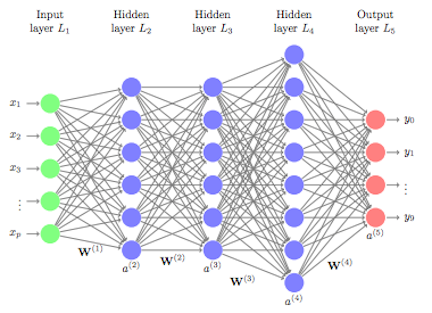
The idea is that we feed our inputs – in this case of independent variables, we then build what are known as hidden layers these layers pass values between them and can start to work out patterns in the data, that as mere mortals we would struggle to analyse. The more layers we expose, the longer the network takes to train due to increase complexity and number of connections. Weights are fed at various stages through the network and then updated through something called back propagation which is normally monitored through an epoch. The network learns through how big an update is made to the weights across the network – this is called learning rate and the loss is optimised and minimised through each pass through the network. How the nodes are activated in the network is controlled by an activation function, which says which nodes to activate and which nodes not to. This network simulates how the human cognitive process learns.
I have reached the end of the theory part of this blog. Let’s get on with implementing it.
Implementing the layers in our network
Firstly we will declare our class and specify the number of inputs to the network:
Lots to explain here:
- The class takes in the Module input – this is the PyTorch module responsible for all the neural network implementation in PyTorch.
- Our parameters in the __init__() constructor are of course self and n_inputs (this is linked to the number of independent or X variables we have in our model.
- Okay, so what the hell is super().__init__()? What this is doing is saying I want to inherit all the parameters from the parent class which in this case will be the ThyroidMLP(Module) parameters. If we didn’t have this, we would have to double type every time we needed to use the Module class. This makes it easier to keep building on top of our original blueprint. The essence of this is that it reduces coding through inheriting parameters. Think of a class of a vehicle there are many types of vehicle, but most would have engines, but your child classes might be a car, motorboat, plane, train – which have massively different behaviours than the parent class.
- The next step is to implement the hidden layers in our network, that we briefly touched on in the theory section. Here we are defining a variable called hidden1 that will act as our first hidden layer, with 10 nodes in it. The layer is a linear layer.
- We then implement a Kaiming Uniform layer to control how the weights of the network get activated. The activation function we define is the popular relu activation.
- We then set our activation function equal to the ReLU (Rectified linear unit) which is a way of suppressing negative weights and allowing for increasing positive weights to activate the nodes in the network.
- This process is repeated for another hidden. The important point to note is that the outputs of the previous layer 1 have to be the inputs to the second layer, notice how hidden1 = Linear(inputs=n_inputs, outputs=10) is then passed forward to the next layer in hidden2.
- The last layer in the network is a Sigmoid curve – which allows the classification to fall between 0 – 1, meaning the higher the weight, the more likely the outcome is 1 = sick, than not sick, or negative in the labels case. Because we are dealing with a binary prediction, a yes and no, we use Sigmoid, otherwise for multiple class labels, we would use a boundary called Softmax.
Create the forward passing mechanism
You will see this in a number of PyTorch scripts – the weights are passed forward through the network and then the updates to the weights i.e. optimization is done by back propogation. Let’s put the final piece of our network together.
We use X to keep passing each layer to the next until we have all of our hidden layers and activation functions defined. We have now created our model class, that we will work with in the training loop.
The full implementation of this part of the class is below:
The fun part is coming up, definition of our training loop.
Step three – the training loop
This is how the model will train and update.
These can be as complex or simple as you want to make them. I have tried to aim it in the middle, as overly simplified would not be useful, and to complicated might fry your brain at this stage, especially if you are a beginner coming at it.
Here we go:
- We have 6 parameters to the model:
- train_dl – this is the dataloader we created earlier
- model – the model to be trained
- Optional parameters:
- epochs – how many times do we want to feed through and back propagate errors (this is an optional parameter as the default is set to 100)
- lr (learning rate) – at what rate the model learns at – too high a value and it misses key updates, too low and it can take forever. This is where the art comes into Machine Learning.
- momentum – is used to speed up training
- save_path – this will be the serialised PyTorch (.pth) file format. All PyTorch models are saved with this postfix.
- The start parameter starts a timer, as we want to time how long our loop takes
- The criterion is how the loss will be calculated. Here we will use binary cross entropy (BCE Loss) for how the loss is computed
- The optimiser – how the loss is minimised via a process called gradient descent. We will use the random gradient descent, or stochastic gradient descent for this
- We default the loss to zero at the start to initialise the variable
The next step is to create the loop to loop through each epoch and start to train the model:
- We use a print statement to print the current epoch
- We set the model to train (model.train()) – this kicks off the training of the model
- We then iterate through our dataloader:
- the optimiser is set to zero gradients, this is important to do, as the gradients can stay in cache and eat up memory
- we pass the inputs into our model at every epoch
- We use: _, preds = torch.max(outputs.data,1) to get the class labels from the outputs variable – which could be renamed to yhat – these are the predictions
- The loss is passed to our chosen criterion – in this instance the binary cross entropy loss we discussed above
- We then set the loss to back propagate through the network updating the weights as it goes i.e. loss.backward()
- Then we need to tell the optimiser to start optimising the next step
- At each step we save the model to a model path using torch.save – here you would want to really implement an if statement to check if this is the best model to save
Note: to use the GPU you would need to cast model.to(device) or model.to(“cuda”) for parallel processing.
There we go we have created the training loop. Next we need to decide how we are going to evaluate the model.
Step four – evaluating the performance of our network
The next function will be used to evaluate our PyTorch model to see if it is any good, or if we have been wasting our time for the last 20 minutes.
The function for this is contained hereunder, and as always, I will add my view of what is happening in each step:
There is a lot to go over here:
- Input parameters to the function are the test_dl dataloader, model the PyTorch model aka ThyroidMLP and a beta value for the metrics section
- We start the function by initialising empty lists for our preds and our ground truth actual labels
- We then loop over the data loader and undertake the following:
- compute the yhat otherwise known as the prediction
- Use the detach().numpy() function to retrieve the weights array from the nd-array
- Set the actual label to a numpy() array
- Reshape the actual to match what we did at the last part of the data loader class
- We then round the predictions
- Finally we append each prediction in the dataloader to the empty list, we also do the same for the actuals
- We use multiple assignment to vstack the predictions and the actuals. This essentially just vertically stacks each one of the predictions in a vertical array i.e. row-wise.
- We then create a confusion matrix (cm) object from sklearn which computes the confusion matrix from the actuals and the predictions – this will tell us how accurate our model is, etc.
- To get each one of the metrics from the array we ravel() the array which takes two separate arrays and produces a continuous flattened arrays. This gives us our True Positive (TP), True Negative (TN), False Positive (FP) and False Negative (FN) statistics.
- From this we build a metrics dictionary with key value pairs, this contains:
- Accuracy – the overall model accuracy
- Area under the ROC curve (AU_ROC) – this is the best evaluation metric to use for imbalanced problems like the thyroid dataset
- F1 score – this is the harmonic mean of the precision and recall
- F-Beta – a variance of the F1 score that allows weighting of a beta value. This is useful if you want to weight your model in one direction, over another. Say you are more interested in precision, than recall, then you would set your beta value greater than 1, if you wanted to use it for precision then the lower beta value the better. There are approaches to selecting the optimal threshold that I won’t cover in this tutorial.
- Matthew’s correlation coefficient – represents the correlation between the true values and the actual values. This is sometimes a more robust metric for working with confusion matrices.
- Precision – the quality of the positive prediction made by the model
- Recall – what proportion of positives were identified correctly
- Included are a number of other metrics computed, such as false discovery rate, false positive rate, misclassification error rate and the confusion matrix values themselves e.g. True Positives, False Positives, False Negatives and True Negatives.
- The final return statement returns the metrics, preds (predictions) and the actuals (actual values).
Step five – creating the prediction routine
This routine is a relatively simple function to those we have compared above. This routine takes in the row (a new list of data) as well as the relevant model and returns a prediction from the model yhat. Finally, we return a detached numpy array:
This will give use a prediction for each input we pass into the model. The next step is to prepare our data ready for working with the model.
Step six – prepare the data to use with our model
We are actually at the point where we will be using our custom model structure to run our model, but first we need an additional helper function to allow us to prepare our dataset:
This function takes the path of where the csv file is stored. In our case this is on GitHub: https://raw.githubusercontent.com/StatsGary/Data/main/thyroid_raw.csv. Then the following happens:
- We use our custom dataloader class entitled ThyroidCSVDataset which has all our processing functions built into a custom class
- We will then use the split_data method we defined in that class to perform a split on our data
- We then create a train and test data loader object – where we are going to shuffle the items in the training set – therefore the results will change on every run.
- Finally, we return the data loaders ready to work with in the modelling task.
Using our custom classes to train the model
We have prepared all the groundwork needed to build out supervised machine learning classifier. So let’s step through and call the relevant functions.
Loading the dataset
We will fetch the thyroid dataset from the blob storage. This dataset is highly imbalanced and is a Kaggle classification project, so I would expect the model to do well in predicting the negative examples and not so well in picking up whether a patient is sick. You would need to have some imbalanced label strategies in your back pocket – such as SMOTE and ROSE, but these are beyond the scope of this tutorial.
Let’s load the data:
Training the model
To train the model we will pass one input – this is the number of independent variables, or predictor variables, to use with the model. I know that the thyroid dataset has 26, so this is the input we would choose. The only thing you would need to change is this value:
To configure the training run we will use the train_model function we created:
Here I pass:
- The train_dl the training data loader used for the model
- The model we initialised at the top i.e. ThyroidMLP
- A path to save the serialised model file to
- Epochs – the number of epochs we want to train over
- The Learning rate i.e. the rate at which the model learns
You will see the epochs running and then you will get a print out of the DAG (Directed acyclic graph).
Evaluating how well the model performs with the test data
Previously we built an evaluation model function, which had a long dictionary of model results. We are going to pass our test dataloader to this to get the results:
To decode this:
- Uses the evaluate_model function to pass in our test data loader, model and specify a beta rate. I want beta to be balanced, so I set 1 as the threshold
- Store the model metrics off the back of the results call to the evaluate model. As the evaluate model has multiple returns, we must specify the zeroth index of the return
- The return will be a dictionary type, so we need to use the from_dict function to convert to a data frame and we specify our column to use as metric. This name could be anything.
- From this conversion our evaluation metric names are actually stored as rows, so we will pull them from the row into a column, give the column a name and reset the indexes of the column
- Finally – I will output these results to a CSV file – using the handy to_csv function.
The results are below:
#                          metric_type      metric
# 0                           accuracy    0.727273
# 1                             AU_ROC    0.497436
# 2                           f1_score    0.096386
# 3            average_precision_score    0.235493
# 4                             f_beta    0.096386
# 5   matthews_correlation_coefficient   -0.008809
# 6                          precision    0.222222
# 7                             recall    0.061538
# 8             true_positive_rate_TPR    0.061538
# 9            false_positive_rate_FPR    0.066667
# 10              false_discovery_rate    0.777778
# 11               false_negative_rate    0.938462
# 12         negative_predictive_value    0.762646
# 13      misclassification_error_rate    0.272727
# 14                       sensitivity    0.061538
# 15                       specificity    0.933333
# 16                                TP   12.000000
# 17                                FP   42.000000
# 18                                FN  183.000000
# 19                                TN  588.000000
As suspected – we have a massively imbalanced datasets, so the MLP is struggling to produce a good classification for the true positives, as the absence of positive labels is apparent.
Let’s poke our model and see what prediction we get, but looking at these results it is most likely to output that the classification of thyroid disease is negative.
Make a prediction against the model
This would be the part where if you were happy you would push the model into production and then new unseen observations would be scored against the model. I will poke it with one observation to see how it performs.
I have used a row in the dataframe where I know the patient is sick to test the label value of the model. I can see that my suspicions about the imbalance in the model are true:
Predicted: 0.499 (class=0)
I would never deploy this model. My next step would be to try some class rebalancing techniques.
Running the model against balanced dataset
For sake of time – I will use a dataset called Ionsphere that I know is well balanced and will show our model in a better light than this example. We will do the data prep and training in one cell and then poke the model. The ionsphere data is stored here:https://raw.githubusercontent.com/StatsGary/Data/main/ion.csv.
Prepare and train
I will add the ionsphere data in one code cell – this will show how to prepare the data, train the model, evaluate and predict against the model:
The only differences here is that I loaded a different dataset and specified the number of input dimensions differently.
Evaluate the model
I have written a little eval_model wrapper function here, as there are a couple of steps to converting the stored dictionary into a data frame:
This returns the metrics data frame, the model metrics as their raw dictionary and the results of the evaluate_model function. Let’s see how our model performs:
#                          metric_type     metric
# 0                           accuracy   0.923810
# 1                             AU_ROC   0.882353
# 2                           f1_score   0.946667
# 3            average_precision_score   0.898734
# 4                             f_beta   0.946667
# 5   matthews_correlation_coefficient   0.829016
# 6                          precision   0.898734
# 7                             recall   1.000000
# 8             true_positive_rate_TPR   1.000000
# 9            false_positive_rate_FPR   0.235294
# 10              false_discovery_rate   0.101266
# 11               false_negative_rate   0.000000
# 12         negative_predictive_value   1.000000
# 13      misclassification_error_rate   0.076190
# 14                       sensitivity   1.000000
# 15                       specificity   0.764706
# 16                                TP  71.000000
# 17                                FP   8.000000
# 18                                FN   0.000000
# 19                                TN  26.000000
This model is much more balanced, and much more unrealistic than the first scenario presented, however it makes for good practice in implemeting the model with different datasets.
Predict with the model
The final step we will make a prediction with the model. I will choose a row that I know should be a positive class and let’s see how our model performs:
Predicted: 0.992 (class=1)
This model does so much better at predicting the right class label.
That is that! You have done excellent!
That is it! You have reached the end of this tutorial. I hope by working through this you feel confident to implement your own PyTorch module, or just use this code for your projects.
Please reach out if you need any help adapting this code. I have really enjoyed putting this together and I continue to develop in this toolset, as I love the flexibility.
All there is left to say is: