

I will take you through step by step how to use the data.table package, and compare it with base R operations, to see the performance gains you get when using this optimised package.
Load in data.table
To load the package in you can follow the below instructions:
1 2 | #install.packages(data.table) library(data.table) |
You should now have everything you need to start the tutorial.
Reading in a data.table csv
To read files in data.table you use the fread syntax to bring files in. I will load the NHSRDatasets package and export this out and then I will use the data.table functionality to read it back in:
1 2 3 4 5 | library(NHSRdatasets) ae <- NHSRdatasets::ae_attendances write.csv(ae, "ae_nhsr.csv", row.names = FALSE) #Set row names to false #Use data.table to read in the document ae_dt <- fread("ae_nhsr.csv") |
This is so much faster than the alternatives. I will show how this compares in the next section, this detracts slightly from the tutorial, but I need to enforce how learning data.table can speed up your R scripts.
Benchmarking the speed of data.table vs Base R
Here, we will create a synthetic frame, using a random number generator, to show how quick the data.table package is compared to base R:
1 2 3 | #Create a random uniform distribution big_data <- data.frame(BigNumbers=runif(matrix(10000000, 10000000))) write.csv(big_data, "bigdata.csv") |
Start the benchmarking after creating the pseudo-massive dataset.
1 2 3 4 5 6 7 8 9 10 11 12 13 14 15 16 | # Start to benchmark using system.time # Read CSV with base base_metrics <- system.time( read.csv("bigdata.csv") ) dt_metrics <- system.time( data.table::fread("bigdata.csv") ) print(base_metrics) print(dt_metrics) # # user system elapsed # 25.78 0.42 26.74 # user system elapsed # 1.09 0.07 0.33 |
To compare this graphically, we will set up a routine to monitor this in ggplot2:
1 2 3 4 5 6 7 8 9 10 11 12 13 14 15 16 17 18 19 20 21 22 23 24 25 26 27 28 29 30 | library(dplyr) library(tibble) library(ggplot2) df <- data.frame( base_run_time = base_metrics[1], #Grab the elapsed time for the user data.table_run_time = dt_metrics[1] #Grab the elapsed time for the user ) #Flip data.frame over to get the run times using transpose df<- data.frame(t(df)) %>% rownames_to_column() %>% setNames(c("Type", "TimeRan")) # Make the ggplot library(ggplot2) plot <- df %>% ggplot(aes(x=Type, y=TimeRan, fill=as.factor(Type))) + geom_bar(stat="identity", width = 0.6) + scale_fill_manual(values= c("#26ACB5", "#FAE920")) + theme_minimal() + theme(legend.position = "none") + coord_flip() + labs(title="Run time comparison data.table and ggpplot", y="Run Time (seconds)", x="Data.Table vs Base", caption="Produced by Gary Hutson") print(plot) |
This shows a marked improvement:
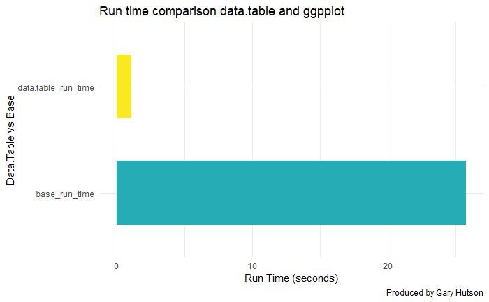
As you can see – data.table is lightening fast compared to base R and it is great for working with large datasets.
We detract, this section is just to highlight how useful the data.table package is for dealing with larger datasets.
Conversion between data.table and data.frame (base) objects
Time to time you may want to convert the data.table objects back to base R, to do this you can follow the below:
1 2 3 4 5 6 7 8 9 10 11 12 13 14 15 | #Convert base data.frame to data.table ae_dt <- as.data.table(ae) class(ae_dt) #Using the setDT command ae_copy <- ae data.table::setDT(ae_copy) class(ae_copy) # Converting this back to a data.frame data.table::setDF(ae_copy) class(ae_copy) # [1] "data.table" "data.frame" # [1] "data.table" "data.frame" # [1] "data.frame" |
Running the class on each of these you can see that the objects have now been converted to the data.table type.
To expand on the above:
- I set the original A and E data, from the loading example, using the as.data.table command, this coerced the data.frame into a data.table object. We inspect that this has been changed by checking the class of the object
- I then made a copy of the data.frame and used the setDT() syntax to set it to a data.table object. Again, I then used class to check the class of the object
- Finally, I used the setDF to force it back to a data.frame, as this object had been converted to a data.table object in the previous step. I used class to check the type and this has successfully been changed back.
Filtering on a data.table object
The general rule to filtering is to use the below visual:
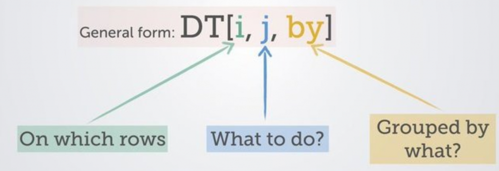
We will used our accident and emergency dataset (ae_dt) from the NHSRDatasets furnished by the NHS-R Community to work with some of the fields and commence filtering:
1 2 3 4 | library(ggplot) # Filter out hospital types and high attendances ae_reduced <- ae_dt[type == 1 & attendances > 30000 & org_code != "R1H", ] #The comma indicates rows and no columns print(ae_reduced) |
This produces:
1 2 3 4 5 6 | # 2019-03-01 RRK 1 32017 10670 10850 # 2019-01-01 RRK 1 31935 12502 11493 # 2018-12-01 RRK 1 30979 8981 11401 # 2018-11-01 RRK 1 30645 8120 11230 # 2018-10-01 RRK 1 30570 7089 10770 # 2018-07-01 RRK 1 32209 6499 11332 |
This selects my arrival type equal to 1, filters out accident and emergency attendances greater than (>) 30000 and organisation code is not equal (!=) to R1H, which relates to a specific NHS trust. The ampersand means filter on this field and(&) that field.
Indexing and Selecting data.table objects
This will show you how to perform selections on columns:
Selecting given columns
The code snippet shows how to select only given columns, as an index:
1 2 3 4 5 6 7 8 9 10 11 12 13 14 15 | #Select by index ae_dt[,1] #Select the first column # Gives: # #period # <date> # 2017-03-01 # 2017-03-01 # 2017-03-01 # 2017-03-01 # 2017-03-01 # 2017-03-01 # 2017-03-01 # 2017-03-01 # 2017-03-01 # 2017-03-01 |
Selecting a vector of columns:
1 2 3 4 5 6 7 8 9 10 11 12 | ae_dt[,c(1,3)] # period type # 2017-03-01 1 # 2017-03-01 2 # 2017-03-01 other # 2017-03-01 1 # 2017-03-01 2 # 2017-03-01 other # 2017-03-01 other # 2017-03-01 other # 2017-03-01 1 # 2017-03-01 other |
Selecting a column by name:
1 2 | head(ae_dt[, period]) #Select by name #[1] "2017-03-01" "2017-03-01" "2017-03-01" "2017-03-01" "2017-03-01" "2017-03-01" |
Selecting multiple columns using a character vector
By character vector, I mean a list of columns to select from the data.frame.
Selecting one column
The example here shows how to select one column:
1 2 3 4 5 6 7 8 9 10 11 12 13 14 15 | # One column my_col <- "period" ae_dt[, my_col, with=FALSE] # period # <date> # 2017-03-01 # 2017-03-01 # 2017-03-01 # 2017-03-01 # 2017-03-01 # 2017-03-01 # 2017-03-01 # 2017-03-01 # 2017-03-01 # 2017-03-01 |
Selecting multiple columns
There are two methods to this. The first:
1 2 3 4 5 6 7 8 9 10 11 12 13 14 15 | #First way ae_dt[, list(period, attendances)] #Returns: # Period Attendances # 2017-03-01 21289 # 2017-03-01 813 # 2017-03-01 2850 # 2017-03-01 30210 # 2017-03-01 807 # 2017-03-01 11352 # 2017-03-01 4381 # 2017-03-01 19562 # 2017-03-01 17414 # 2017-03-01 7817 |
The second method has the same result, but looks cleaner than the previous method:
1 | ae_dt[, .(period, attendances)] |
This is personal choice, but the .() method works best for me. Again, personal preference.
Dropping columns
To drop columns in a data.table you can do it with a character vector, as below:
1 2 3 4 5 6 7 8 | ae_dt_copy <- ae_dt drop_cols <- c("period", "breaches") #Specify columns to drop ae_dt_copy[, !drop_cols, with=FALSE] # This says keep the columns that are not equal to ! my list of drop cols names(ae_drops) #The result: #[1] "month" "org_code" "type" "attendances" "breaches" "admissions" |
Renaming columns
To rename columns, use this convention below:
1 2 3 4 5 | # Rename a single column setnames(ae_dt_copy, "period", "month", skip_absent = TRUE) colnames(ae_dt_copy) #Results in: #[1] "month" "org_code" "type" "attendances" "breaches" "admissions" |
Viola, there you go, renamed from old to new.
Column creation from existing columns like mutate
To create a new column in base you use the dollar sign, to do it in dplyr you use mutate and in data.table you use the below conventions in the sub sections.
Creating one new column
1 2 3 4 5 6 7 8 9 10 11 12 13 | new_col <- ae_dt_copy[, ed_performance := 1-(breaches/attendances)] glimpse(new_col) #Results in: #Rows: 12,765 #Columns: 7 #$ month <date> 2017-03-01, 2017-03-01, 2017-03-01, 2017-03-01, 2017-03-01, 2017-03-01, 2017-03-01, 2017-03-01, 2017-03-01, 2017-~ #$ org_code <fct> RF4, RF4, RF4, R1H, R1H, R1H, AD913, RYX, RQM, RQM, RJ6, RJ6, Y02696, NX122, RVR, RVR, RJ1, RJ1, RJ1, Y03082, RQX,~ #$ type <fct> 1, 2, other, 1, 2, other, other, other, 1, other, 1, other, other, other, 1, 2, 1, 2, other, other, 1, other, 1, 2~ #$ attendances <dbl> 21289, 813, 2850, 30210, 807, 11352, 4381, 19562, 17414, 7817, 6654, 3844, 1069, 2147, 12649, 544, 12385, 832, 293~ #$ breaches <dbl> 2879, 22, 6, 5902, 11, 136, 2, 258, 2030, 86, 1322, 140, 0, 0, 473, 5, 2092, 0, 5, 0, 635, 0, 2632, 68, 190, 4153,~ #$ admissions <dbl> 5060, 0, 0, 6943, 0, 0, 0, 0, 3597, 0, 2202, 0, 0, 0, 3360, 7, 3181, 0, 0, 0, 1684, 0, 3270, 12, 0, 4477, 0, 0, 18~ #$ ed_performance <dbl> 0.8647658, 0.9729397, 0.9978947, 0.8046342, 0.9863693, 0.9880197, 0.9995435, 0.9868112, 0.8834271, 0.9889983, 0.80~ |
This shows that the new column ED performance has been added to the data.
Creating multiple columns
To create multiple columns, use this convention:
1 2 3 4 5 6 7 8 9 10 11 12 13 14 15 16 17 | mult_cols <- ae_dt_copy[, `:=` (ed_performance_inv = breaches/attendances, admit_to_attend_ratio = admissions/attendances)] glimpse(mult_cols) #Results in: # Rows: 12,765 # Columns: 9 # $ month <date> 2017-03-01, 2017-03-01, 2017-03-01, 2017-03-01, 2017-03-01, 2017-03-01, 2017-03-01, 2017-03-01, 2017-03-01~ # $ org_code <fct> RF4, RF4, RF4, R1H, R1H, R1H, AD913, RYX, RQM, RQM, RJ6, RJ6, Y02696, NX122, RVR, RVR, RJ1, RJ1, RJ1, Y0308~ # $ type <fct> 1, 2, other, 1, 2, other, other, other, 1, other, 1, other, other, other, 1, 2, 1, 2, other, other, 1, othe~ # $ attendances <dbl> 21289, 813, 2850, 30210, 807, 11352, 4381, 19562, 17414, 7817, 6654, 3844, 1069, 2147, 12649, 544, 12385, 8~ # $ breaches <dbl> 2879, 22, 6, 5902, 11, 136, 2, 258, 2030, 86, 1322, 140, 0, 0, 473, 5, 2092, 0, 5, 0, 635, 0, 2632, 68, 190~ # $ admissions <dbl> 5060, 0, 0, 6943, 0, 0, 0, 0, 3597, 0, 2202, 0, 0, 0, 3360, 7, 3181, 0, 0, 0, 1684, 0, 3270, 12, 0, 4477, 0~ # $ ed_performance <dbl> 0.8647658, 0.9729397, 0.9978947, 0.8046342, 0.9863693, 0.9880197, 0.9995435, 0.9868112, 0.8834271, 0.988998~ # $ ed_performance_inv <dbl> 0.1352341585, 0.0270602706, 0.0021052632, 0.1953657729, 0.0136307311, 0.0119802678, 0.0004565168, 0.0131888~ # $ admit_to_attend_ratio <dbl> 0.237681432, 0.000000000, 0.000000000, 0.229824561, 0.000000000, 0.000000000, 0.000000000, 0.000000000, 0.2~ |
That is how you do it in data.table.
Grouping with group_by in data.table
Suppose I want to create a summary frame, similar to group_by() and summarise() in dplyr. This can be achieved in data.table, like below:
1 2 3 4 5 6 7 8 9 10 11 12 13 14 15 | summary_frame <- ae_dt_copy[, .(mean_attendance=mean(attendances), mean_breaches=mean(breaches), sum_attendances=sum(attendances)), by=.(org_code)] glimpse(summary_frame) #Results in: # Rows: 274 # Columns: 4 # $ org_code <fct> RF4, R1H, AD913, RYX, RQM, RJ6, Y02696, NX122, RVR, RJ1, Y03082, RQX, RY9, RYJ, RJZ, RAX, RJ2, R1K, RP6, RAT, RAP~ # $ mean_attendance <dbl> 8091.7500, 13625.7500, 4437.1944, 18374.1111, 12686.6667, 7251.8056, 1104.9167, 2547.0000, 5437.7000, 5493.8704, ~ # $ mean_breaches <dbl> 1.403667e+03, 1.897444e+03, 1.555556e+00, 1.647222e+02, 7.678056e+02, 8.867778e+02, 0.000000e+00, 0.000000e+00, 3~ # $ sum_attendances <dbl> 873909, 1471581, 159739, 661468, 913440, 522130, 39777, 30564, 489393, 593338, 133587, 370767, 162800, 868344, 85~ |
This shows that the relevant summary stats have been created and it has been grouped by our grouping factor, in this case it is the organisation code. See NHSDataDictionaRy package for full list of lookups.
Chaining in data.table – similar to Magrittr’s pipe operator (%>%)
Chaining in data.table can be achieved by the following:
1 2 3 4 5 6 7 8 9 10 11 12 13 14 15 16 | chained <- ae_dt_copy[, .(mean_attendance=mean(attendances), mean_breaches=mean(breaches), sum_attendances=sum(attendances)), by=.(org_code)][order(org_code)] # Adding square brackets, instead of %>%, chains the ordering # Here we create a group by and summarise function and at the end we add another # Command sequence i.e. group by org code, summarise the mean and then order by ord code glimpse(chained) #Show ordering by org_code: # Rows: 274 # Columns: 4 # $ org_code <fct> 8J094, AAH, AC008, AD913, AF002, AF003, AJN, ATQ02, AXG, AXT02, C82009, C82010, C82038, C83023, DD401, E84068, E8~ # $ mean_attendance <dbl> 2857.8077, 189.1111, 1032.3200, 4437.1944, 628.5000, 503.8333, 761.8056, 3540.1389, 3040.5000, 3522.9200, 341.222~ # $ mean_breaches <dbl> 0.00000000, 0.05555556, 0.76000000, 1.55555556, 0.00000000, 0.00000000, 0.00000000, 0.00000000, 31.83333333, 0.00~ # $ sum_attendances <dbl> 74303, 6808, 25808, 159739, 7542, 6046, 27425, 127445, 36486, 88073, 12284, 10566, 10996, 12530, 30910, 96066, 26~ |
What is .SD and why should I care
Let’s suppose, you want to compute the mean of all the variables, grouped by ‘org_code’. How to do that?
You can create the columns one by one by writing by hand. Or, you can use the lapply() function to do it all in one go. But lapply() takes the data.frame as the first argument. Then, how to use `lapply() inside a data.table?
1 2 3 4 5 6 7 8 9 10 | ae_summarised <- ae_dt_copy[, lapply(.SD[, 4:6, with=F], mean), by=org_code] # .SD allows for it to be used in an lapply statement to create the column mean group by org_code # of multiple columns glimpse(ae_summarised) # Rows: 274 # Columns: 4 # $ org_code <fct> RF4, R1H, AD913, RYX, RQM, RJ6, Y02696, NX122, RVR, RJ1, Y03082, RQX, RY9, RYJ, RJZ, RAX, RJ2, R1K, RP6, RAT, RAP,~ # $ breaches <dbl> 1.403667e+03, 1.897444e+03, 1.555556e+00, 1.647222e+02, 7.678056e+02, 8.867778e+02, 0.000000e+00, 0.000000e+00, 3.~ # $ admissions <dbl> 1556.87037, 2404.24074, 0.00000, 0.00000, 1868.90278, 1018.13889, 0.00000, 0.00000, 1326.80000, 1093.26852, 0.0000~ # $ ed_performance <dbl> 0.9217378, 0.9263262, 0.9996570, 0.9910515, 0.9529410, 0.8655493, 1.0000000, 1.0000000, 0.9692298, 0.9472967, 0.97~ |
Adding .SDCols to the mix
Instead of me slicing the breaches to ed_performance column – I could add .SDcols to specify the exact columns to use in the function:
1 2 3 4 5 6 7 8 9 10 11 12 | sd_cols_agg <- ae_dt_copy[, lapply(.SD, mean), by=org_code, .SDcols=c("breaches", "admissions")] # Take the mean, group by organisation code and use SDCols breaches and admissions to performs aggregations on glimpse(sd_cols_agg) # RESULTS # Rows: 274 # Columns: 3 # $ org_code <fct> RF4, R1H, AD913, RYX, RQM, RJ6, Y02696, NX122, RVR, RJ1, Y03082, RQX, RY9, RYJ, RJZ, RAX, RJ2, R1K, RP6, RAT, RAP, Y02~ # $ breaches <dbl> 1.403667e+03, 1.897444e+03, 1.555556e+00, 1.647222e+02, 7.678056e+02, 8.867778e+02, 0.000000e+00, 0.000000e+00, 3.7044~ # $ admissions <dbl> 1556.87037, 2404.24074, 0.00000, 0.00000, 1868.90278, 1018.13889, 0.00000, 0.00000, 1326.80000, 1093.26852, 0.00000, 1~ |
It takes some getting used to for tidyverse users, but the performance benefits are massive.
Setting Keys – to speed up searches
Setting one or more keys on a data.table enables it to perform binary search, which is many order of magnitudes faster than linear search, especially for large data. To set keys, follow the routine below:
1 2 3 4 | setkey(ae_dt_copy, org_code) # Check the key has been assigned key(ae_dt_copy) #Prints out org_code as the key #[1] "org_code" |
Merging tables with keys is soooo much faster
This will now allow me to merge tables with ease on the new key, which is the organisation code identifier:
1 2 3 4 5 6 7 8 9 10 11 12 13 | dt1 <- ae_dt_copy[, .(org_code, breaches, admissions)] dt2 <- ae_dt_copy[1:10, .(org_code, type)] # Join the tables merged <- dt1[dt2] glimpse(merged) # RESULTS Rows: 260 Columns: 4 $ org_code <fct> 8J094, 8J094, 8J094, 8J094, 8J094, 8J094, 8J094, 8J094, 8J094, 8J094, 8J094, 8J094, 8J094, 8J094, 8J094, 8J094, 8J094,~ $ breaches <dbl> 0, 0, 0, 0, 0, 0, 0, 0, 0, 0, 0, 0, 0, 0, 0, 0, 0, 0, 0, 0, 0, 0, 0, 0, 0, 0, 0, 0, 0, 0, 0, 0, 0, 0, 0, 0, 0, 0, 0, 0~ $ admissions <dbl> 0, 0, 0, 0, 0, 0, 0, 0, 0, 0, 0, 0, 0, 0, 0, 0, 0, 0, 0, 0, 0, 0, 0, 0, 0, 0, 0, 0, 0, 0, 0, 0, 0, 0, 0, 0, 0, 0, 0, 0~ $ type <fct> other, other, other, other, other, other, other, other, other, other, other, other, other, other, other, other, other,~ |
Removing keys
To remove the keys the process is pretty similar to the key creation steps:
1 2 | setkey(ae_dt_copy, NULL) key(ae_dt_copy) |
This will output NULL, as the key has been unassigned.
Joining tables with merge
To recap, table joins can take a number of forms, but in R they are done by using the merge statement.
Next, I show how data.table handles joining tables. First, I will set up the data.table:
1 2 | dt1 <- ae_summarised dt2 <- ae_summarised[1:10, .(org_code, new_admits=admissions)] |
Inner join – only matching rows count from both tables
The visual below shows what this does:
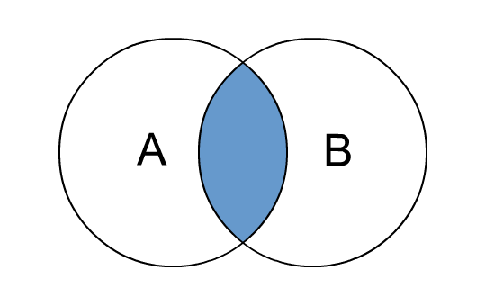
Give me the intersection between table A and B i.e. the records that match:
1 2 3 4 5 6 7 8 9 10 | inner_joined_df <- merge(dt1, dt2, by="org_code") glimpse(inner_joined_df) #RESULTS # Rows: 10 # Columns: 5 # $ org_code <fct> AD913, NX122, R1H, RF4, RJ1, RJ6, RQM, RVR, RYX, Y02696 # $ breaches <dbl> 1.555556, 0.000000, 1897.444444, 1403.666667, 667.203704, 886.777778, 767.805556, 370.444444, 164.722222, 0.000000 # $ admissions <dbl> 0.000, 0.000, 2404.241, 1556.870, 1093.269, 1018.139, 1868.903, 1326.800, 0.000, 0.000 # $ ed_performance <dbl> 0.9996570, 1.0000000, 0.9263262, 0.9217378, 0.9472967, 0.8655493, 0.9529410, 0.9692298, 0.9910515, 1.0000000 # $ new_admits <dbl> 0.000, 0.000, 2404.241, 1556.870, 1093.269, 1018.139, 1868.903, 1326.800, 0.000, 0.000 |
You can see that only 10 rows have been matched, as the aggregate table is a subset of the organisation codes (org_codes).
Left join – all records from the left side and only those matching on the right
This can be visualised as:
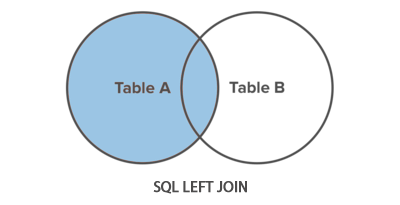
To implement with merge statement:
1 2 3 4 5 6 7 8 9 10 | left_joined <- merge(dt1, dt2, by="org_code", all.x = TRUE, allow.cartesian = FALSE) glimpse(left_joined) #RESULTS Rows: 274 Columns: 5 $ org_code <fct> 8J094, AAH, AC008, AD913, AF002, AF003, AJN, ATQ02, AXG, AXT02, C82009, C82010, C82038, C83023, DD401, E84068, E84~ $ breaches <dbl> 0.00000000, 0.05555556, 0.76000000, 1.55555556, 0.00000000, 0.00000000, 0.00000000, 0.00000000, 31.83333333, 0.000~ $ admissions <dbl> 0.000000, 0.000000, 0.000000, 0.000000, 0.000000, 0.000000, 0.000000, 1.416667, 0.000000, 0.000000, 0.000000, 0.00~ $ ed_performance <dbl> 1.0000000, 0.9996942, 0.9992052, 0.9996570, 1.0000000, 1.0000000, 1.0000000, 1.0000000, 0.9900759, 1.0000000, 1.00~ $ new_admits <dbl> NA, NA, NA, 0, NA, NA, NA, NA, NA, NA, NA, NA, NA, NA, NA, NA, NA, NA, NA, NA, NA, NA, NA, NA, NA, NA, NA, NA, NA,~ |
We see NAs coming to play, as there is not a match from the right table, but all the data from the left table is retained. Violla!
Outer join – return all records that match from both tables
An outer join can be visualised below:
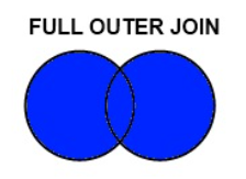
To implement this with the merge statement in R:
1 2 3 4 5 6 7 8 9 10 | outer_join <- merge(dt1, dt2, by="org_code", all=TRUE) glimpse(outer_join) #RESULTS Rows: 274 Columns: 5 $ org_code <fct> 8J094, AAH, AC008, AD913, AF002, AF003, AJN, ATQ02, AXG, AXT02, C82009, C82010, C82038, C83023, DD401, E84068, E84~ $ breaches <dbl> 0.00000000, 0.05555556, 0.76000000, 1.55555556, 0.00000000, 0.00000000, 0.00000000, 0.00000000, 31.83333333, 0.000~ $ admissions <dbl> 0.000000, 0.000000, 0.000000, 0.000000, 0.000000, 0.000000, 0.000000, 1.416667, 0.000000, 0.000000, 0.000000, 0.00~ $ ed_performance <dbl> 1.0000000, 0.9996942, 0.9992052, 0.9996570, 1.0000000, 1.0000000, 1.0000000, 1.0000000, 0.9900759, 1.0000000, 1.00~ $ new_admits <dbl> NA, NA, NA, 0, NA, NA, NA, NA, NA, NA, NA, NA, NA, NA, NA, NA, NA, NA, NA, NA, NA, NA, NA, NA, NA, NA, NA, NA, NA,~ |
That concludes the joins section. The final section will look at pivoting, the data.table way!
Pivots, alas more pivots
This example uses the copy data frame we made and uses the organisation code by the type of attendances. I want to then summarise the mean admissions by type and organisation code.
Pivots can be implemented in data.table in the following way:
1 2 3 4 5 6 7 8 9 10 11 12 13 | dcast.data.table(ae_dt_copy, org_code ~ type, fun.aggregate = mean, value.var = 'admissions') #RESULTS # org_code 1 2 other # RYR 3418.0556 NaN 0.000000e+00 # RYW NaN 0.00000000 NaN # RYX NaN NaN 0.000000e+00 # RYY NaN NaN 0.000000e+00 # Y00058 NaN NaN 0.000000e+00 # Y00751 NaN NaN 0.000000e+00 # Y01069 NaN NaN 0.000000e+00 # Y01231 NaN NaN 0.000000e+00 # Y02147 NaN NaN 0.000000e+00 # Y02428 NaN NaN 0.000000e+00 |
Final thoughts
Data.table is a powerhouse when it comes to speeding up your computations and script. It is one of those must learn packages and I hope this tutorial has given you the interest to try and adapt your code to run more quickly, using the data.table way.
For the vignette [<– click here]. To access content via GitHub.
Happy wrangling!!!!
Thanks for this. But why not using fwrite instead of write.csv, especially when you use fread?!? It’s much much faster.
Yes, very good point. Perhaps haste? Fwrite would have certainly sped up the process. Thanks for the spot.
I have a question – I have the following data.table:
i t TRH pTSH TSH TT4 FT4 TT3 FT3 cT3 V11
1: NA day h:m:s ng/l mU/l mU/l nmol/l pmol/l nmol/l pmol/l pmol/l NA
2: 1 1900-01-01 00:00:00 2500.00 4.00 55.4294 44.1721 6.4008 1.8639 3.1013 4283.5034 NA
3: 2 1900-01-01 00:01:40 2720.2094 4.00 55.4294 44.1721 6.4008 1.8639 3.1013 4283.5034 NA
4: 3 1900-01-01 00:03:20 2739.5253 4.00 57.4004 44.1721 6.4008 1.8639 3.1013 4283.5034 NA
5: 4 1900-01-01 00:05:00 2335.1469 4.00 59.3463 44.1721 6.4008 1.8639 3.1013 4283.5034 NA
6: 5 1900-01-01 00:06:40 3187.1927 4.00 60.826 44.1721 6.4008 1.8639 3.1013 4283.5034 NA
As you can see I have the first two rows as headers (and would like to keep them in one line) So how do I convert them to a one-line header?