
What is DPLYR?
Dplyr is a grammar of data manipulation, providing a consistent set of verbs that help you solve the most common data manipulation challenges. The next series of examples will show how you can use the shortcuts in Dplyr to achieve the results of traditional R data manipulation, but faster.
Setting dplyr up in your R environment
To install dplyr you must use the install.packages(“dplyr”) command in your R script. However, the current trend is to use the tidyverse that contains more than just dplyr. The image below shows all the associated packages available to the tidyverse and is another genius invention of Hadley Wickham:
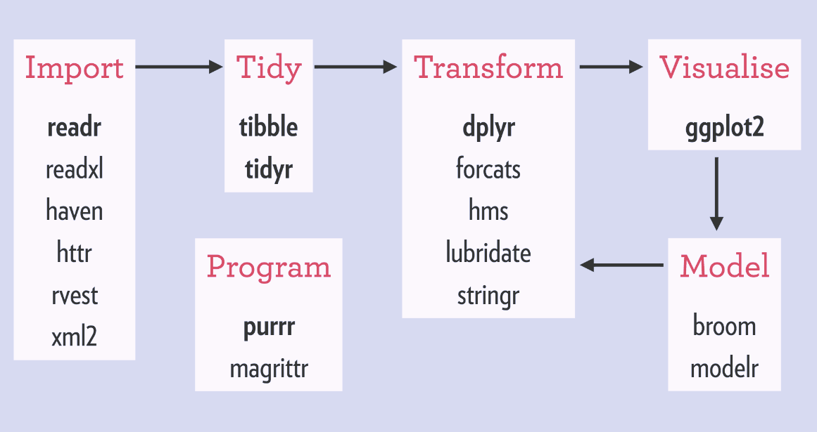
Source: https://rviews.rstudio.com/2017/06/08/what-is-the-tidyverse/
The code below is how to install this simply in R:
1 2 | install.packages("tidyverse") library(tidyverse) |
Getting the test data set up
The test data is an attachment (in .csv format) stored on this website. To read this into R we are going to use the read_csv command (taken from the enhanced import functionality powered by the tidyverse and in particular, the package readr) with this URL to force R to read directly into the application. This can be achieved by following the steps hereunder:
1 2 3 | OPdf <- read.csv("https://hutsons-hacks.info/wp-content/uploads/2018/05/DPLYR.csv", header = TRUE) str(OPdf) |
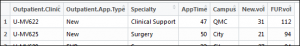
The data has a couple of fields (completely make at random) to show: outpatient clinic, outpatient appointment type; clinical specialty of the outpatient clinic; how long the appointment lasted – in minutes; the campus; the volume of new appointments associated to that clinic and the volume of outpatient follow ups. The next series of tutorials will show how to use dplyr and its functionality to easily manipulate the data.
Filtering with DPLYR via the Tidyverse
To filter in DPLYR we use the filter() command:
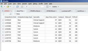
1 2 | dplyrFilter <- filter(OPdf, Campus=="QMC", Specialty!="Surgery", OPdf$New.vol > 30) |
This says create a data frame called tidy_filter and filter from the existing data frame. Then, I only want to return records where the Campus is equal to (==) QMC; where the Specialty is not equal (!=) to Surgery and with a new outpatient volume greater than 30. This will give me the lists of clinics matching that description. You will be able to see this new data frame in your R Studio Environment window. By clicking this you will see that the data frame has reduced down to 8 observations from 48:
The traditional and R native way would be to use something similar to:
1 | tradFilter <- OPdf[OPdf$Campus=="QMC" & OPdf$Specialty!="Surgery" & OPdf$New.vol >30,] |
As you can see – the dplyr method is much easier to use.
Slicing a data frame with DPLYR
Slicing is a way to reduce the number of records in a data frame. This can easily be achieved by using the following syntax:
1 | DPLYRSlice <- slice(OPdf, 1:10) |
This would take the first 10 records of the existing data frame (OPdf) and store them in the relevant named data frame, in this instance DPLYRSlice.
Arranging data frames with DPLYR
You can arrange a data frame in two ways:
1 2 | ascendingOrder <- arrange(OPdf, Campus, Specialty, New.vol) descendingOrder <- arrange(OPdf, desc(New.vol)) |
You can arrange a data frame in two ways descending and ascending. The ascendingOrder data frame uses the arrange() function to arrange the existing data frame (always the first parameter passed to the function) alongside Campus, Specialty and New.vol to achieve a sorting hierarchy, as displayed hereunder:
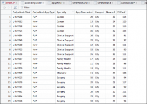
This shows that it has been sorted in the order stipulated i.e. Campus first and then the other fields passed in the prior paragraph.
Using DPLYR like SQL – SELECT statement
This function is very powerful for selecting a sub set of your data:
1 2 3 | DPLYRSelect <- select(OPdf, Specialty, Campus) #Selects specialty and campus and drops all other fields DPLYRSelect |
Resulting in a new data frame with only the Specialty and Campus fields contained.
Renaming columns with DPLYR
Renaming columns is easy in DPLYR, just see:
1 | DPLYRRename <- rename(OPdf, AppTime = App.Time..mins.) |
This takes the existing column name of App.Time..mins. and renames it to AppTime. This new column can now be seen in the data frame:
Performing a SELECT Distinct with DPLYR
Another function, if you are familiar with SQL, will be the SELECT Distinct function:
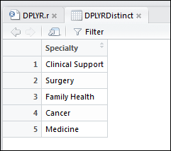
1 | DPLYRDistinct <- distinct(select(OPdf, Specialty)) |
This will return a table of only the distinct clinical specialties in our trust:
Mutating in DPLYR
This sounds fancy, in saying that, it is only an way to use existing columns to perform some sort of aggreation or function. This adds a column and stores the result. Here I will calculate something called a follow up to new outpatient ratio:
1 | DPLYRMutate <- mutate(OPdf, mut_col=FUP.vol/New.vol) |
You may ask – what has this achieved? What has happened here is a new column has been created called mut_col and then I have performed a division on the follow up volume compared to the new volume. These volumes relate to how many new and follow up patients each of our outpatient clinics has seen. The result:
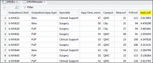
This now has the ratio I require in a new data frame.
Using Transmute in DPLYR
Even more puzzled? This is a way to perform the same aggregation or function, as mutate, but to only return the values of the function and nothing else. Clear as mud? Have a look below:
1 | DPLYRTransmute <- transmute(OPdf, mut_col=FUP.vol/New.vol) |
The syntax looks very similar, but the resultant output is very different:
![]()
As you can observe, all that has been returned is the calculated field or column and nothing else. This is the purpose of transmute.
Use Case When instead of ifelse with DPLYR
Case when will be familiar to all SQL users, especially those who favour the Microsoft offering. I like this function as it can be used with transmute() to add a calculated column:
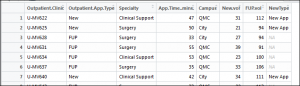
1 2 | CaseWhen <- mutate(OPdf, NewType=case_when(OPdf$Outpatient.App.Type == "New" ~ "New App")) |
In summary, this function uses mutate and the existing data frame to create a new field. Then, it uses the appointment type where it is a new appointment to set a new value, or this could be used to flag values with a binary marker. The result will be a new column called NewType:
Using SQL Inner, Left, Right and Outer Join
DPLYR has implementations of all these join types. Please refer to the guidance created by Hadley Wickham (creator of DPLYR).
Summarise function with DPLYR
DPLYR contains a function, which allows you to summarise the information contained within a data frame:
1 2 | summariseDF <- summarise(OPdf, avg_new_OP=mean(New.vol, na.rm = TRUE)) |
This performs a mean average on the new outpatient volumes and removes NA values using the na.rm=TRUE.
Sampling a data frame in DPLYR
There are a number of functions for taking a sample from a data frame in DPLYR. The two methods I show here are the percentage sample and the volume sample methods. The syntax for these can be seen here:
1 2 3 4 5 | #-------------------Sampling the data frame with DPLYR------------------- OPdf24Rand <- sample_n(OPdf, 24) #Take 24 random samples of the dataframe OPdfPercRand <- sample_frac(OPdf,0.10) #Give me a sample of 24 percent of the data |
These functions are relatively self explanatory. They take an existing data frame and sample relating to the parameters passed to it.
Conclusion
DPLYR is extremely powerful. These are just a few of my favourtie functions to use, conversely there are a number that I have not detailed in this post. Again, if you need a point of reference, then this DPLYR guide is the essential reference.
Happy DPLYRing!